
01Your model performs very well on training data but poorly on validation and test data. What is happening, how would you diagnose it, and how would you fix it?
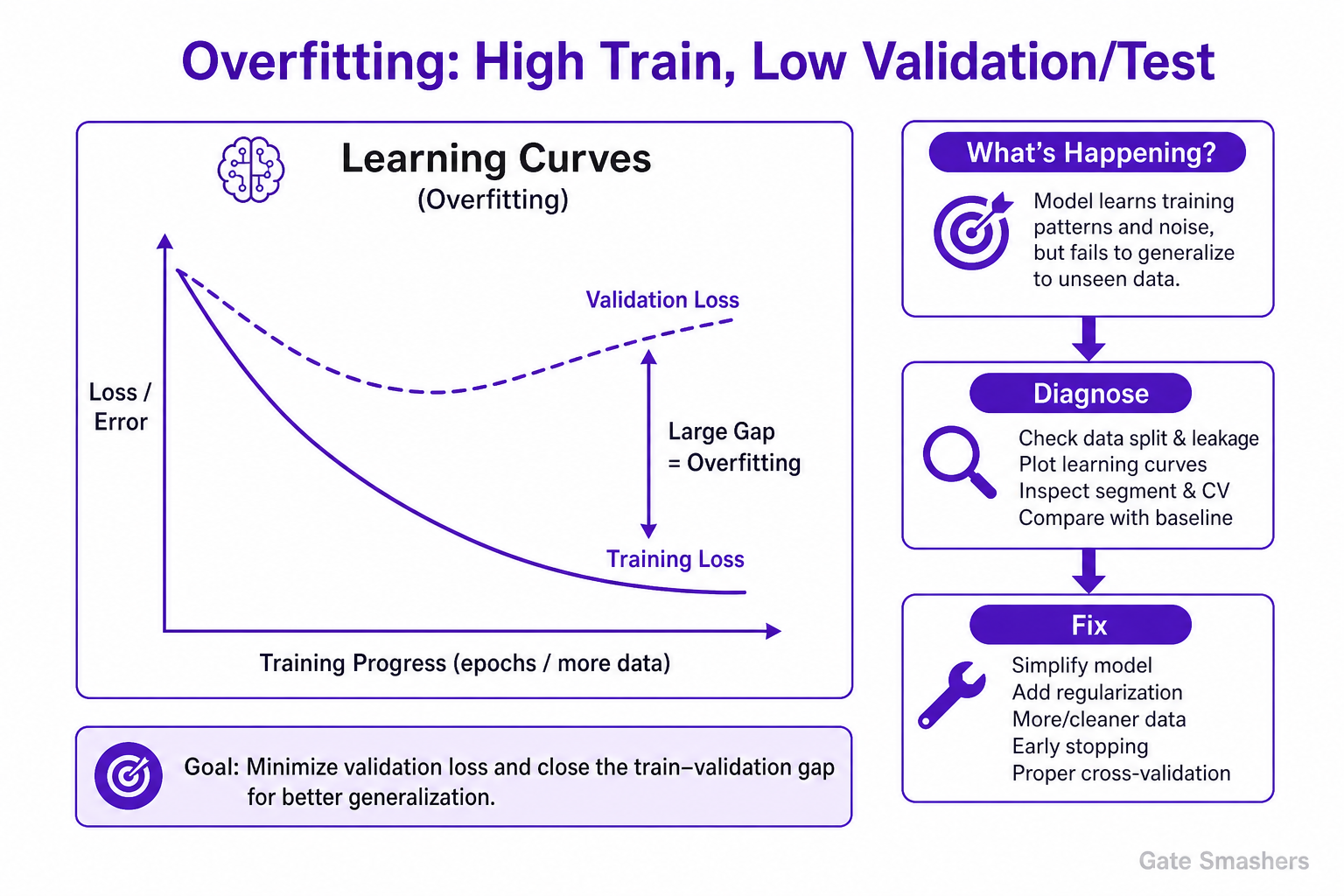
This is usually overfitting: the model has learned patterns and noise specific to the training set but does not generalize to unseen data. I would first verify the data split and rule out leakage, then compare training and validation learning curves. Depending on the cause, I would simplify the model, add regularization, collect or augment data, use early stopping, improve cross-validation, or reduce noisy features. I would confirm the fix using an untouched test set rather than the training score.
| Observation | Likely interpretation | Next check or action |
|---|---|---|
| Low training error, high validation error | High variance / overfitting | Learning curves, regularization, simpler model |
| Both training and validation errors are high | High bias / underfitting | More capacity, better features, less regularization |
| Validation is unexpectedly excellent | Possible leakage or duplicate samples | Audit features and split boundaries |
| Offline score is good, production score is poor | Distribution or pipeline mismatch | Compare live features, labels and segments |
A persistently large positive validation-loss gap is a practical signal of overfitting, although leakage and split problems must still be ruled out.
Recognising the pattern
Overfitting is a generalization problem. A very low training error with a much higher validation error indicates that the model has enough capacity to fit the training examples but has learned relationships that do not remain stable on unseen data. A large train–validation gap is evidence of high variance, but it is not enough by itself to identify the root cause.
Diagnose before changing the model
- Check the split: Ensure duplicate users, repeated events, future information and related samples do not appear across training and validation sets.
- Plot learning curves: Compare training and validation loss as the number of training examples or epochs increases. A widening validation gap is a strong overfitting signal.
- Inspect segment performance: Evaluate important classes, user groups, time periods and rare cases separately. A good average metric may hide weak generalization.
- Compare cross-validation folds: Large variation between folds may indicate limited data, unstable features or a non-representative split.
- Establish a baseline: Compare the complex model with a simpler linear model, shallow tree or business-rule baseline.
Corrective actions
- Reduce variance: Use a simpler architecture, shallower trees, fewer parameters or fewer noisy features.
- Regularize: Apply L1/L2 penalties, dropout, pruning, minimum leaf sizes or other model-appropriate constraints.
- Improve the data: Collect more representative examples, fix label noise and use valid augmentation where the domain permits it.
- Stop at the right time: Monitor validation loss and restore the best checkpoint with early stopping.
- Tune correctly: Perform model selection inside cross-validation and keep the final test set untouched.
Important interview distinction
More training data often helps high variance, but it does not repair leakage, a wrong objective or a train–production mismatch. Regularization also creates a trade-off: too much can move the model from high variance to high bias.
Practical example
Suppose a fraud model achieves 99% training accuracy and 84% validation accuracy. Before reducing the neural network, check whether transactions from the same customer were split across datasets or whether a post-transaction feature reveals the label. If the split is clean, compare learning curves, regularize the model and evaluate precision–recall metrics on an untouched time-based test set.
02Explain bias versus variance. How do you identify which problem a model has, and how do you choose the right remedy?
Bias is error caused by assumptions that are too simple, while variance is sensitivity to the particular training sample. High-bias models underfit and usually perform poorly on both training and validation data. High-variance models fit training data well but perform much worse on validation data. I diagnose them using training and validation errors, learning curves and cross-validation stability, then adjust capacity, features, regularization and data accordingly.
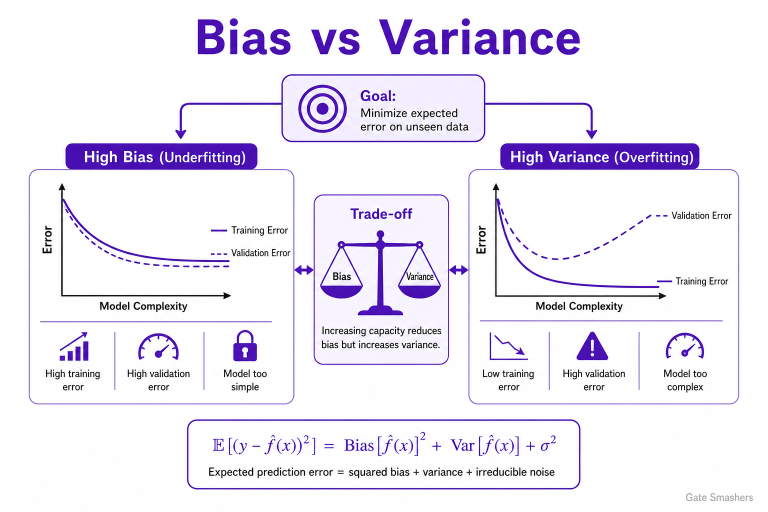
Expected prediction error can be viewed as squared bias, variance and irreducible noise. The exact decomposition shown applies to squared-error regression.
Core idea
Bias and variance describe two different ways a model can fail to generalize. Bias comes from an overly restricted model or representation that cannot capture the real relationship. Variance comes from a model that reacts too strongly to the details or noise of its training sample.
How to diagnose them
- High bias: Training performance is already weak, and validation performance is similarly weak. Adding more data alone usually gives limited improvement because the model cannot fit the underlying pattern.
- High variance: Training performance is strong, but validation performance is significantly worse. Performance may also vary widely across cross-validation folds.
- Both: A real system can have high bias in one segment and high variance in another. Inspect slices rather than relying only on a global metric.
How to reduce high bias
- Use a more expressive model or richer feature representation.
- Reduce excessive regularization.
- Train longer when optimization has not converged.
- Add meaningful interactions, nonlinear features or domain knowledge.
- Verify that the target and loss function represent the actual task.
How to reduce high variance
- Add more representative training data.
- Simplify the model or constrain its depth and capacity.
- Increase appropriate regularization.
- Remove unstable or noisy features.
- Use bagging, early stopping or robust cross-validation.
Important interview point
The goal is not to minimize bias or variance independently. The goal is to minimize expected error on unseen data. Increasing model capacity may reduce bias but increase variance, while strong regularization may reduce variance but increase bias.
03Why do we use training, validation and test sets, and how can data leakage occur between them?
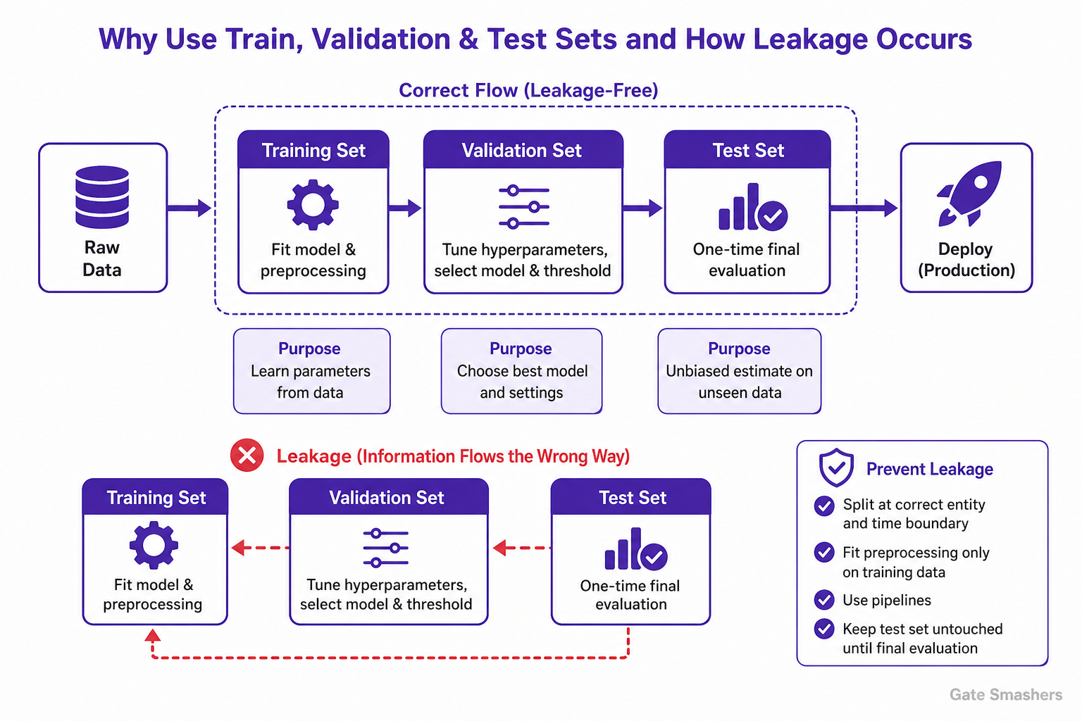
The training set fits model parameters, the validation set supports model selection and hyperparameter tuning, and the test set provides a final unbiased estimate after all choices are fixed. Leakage occurs when information unavailable at prediction time, or information from validation/test data, influences training. I prevent it by splitting at the correct entity and time boundary, fitting every preprocessing step only on training data, using pipelines, and keeping the test set untouched until final evaluation.
| Split | Used for | Must not be used for |
|---|---|---|
| Training | Fit model and preprocessing parameters | Final performance claim |
| Validation | Tune hyperparameters, select models and thresholds | Direct parameter fitting |
| Test | One-time final evaluation of the frozen pipeline | Repeated tuning or feature selection |
Purpose of each split
The three splits answer different questions. Training data asks, ‘Can the algorithm learn parameters?’ Validation data asks, ‘Which model and settings should we choose?’ Test data asks, ‘How well should the final frozen procedure generalize to unseen data?’ Repeatedly checking the test result during development turns the test set into another validation set.
Common leakage paths
- Preprocessing leakage: Scaling, imputing, feature selection or dimensionality reduction is fitted before splitting, so statistics from held-out data enter training.
- Target leakage: A feature contains the target directly or contains information created after the outcome occurred.
- Entity leakage: Records for the same user, patient, device or document appear in different splits.
- Temporal leakage: Future observations or future aggregates are used to predict an earlier event.
- Tuning leakage: The test set influences hyperparameters, thresholds, features or model choice.
- Augmentation leakage: Near-duplicate augmented versions of one source example cross split boundaries.
Safe workflow
- Define the real prediction time and the information available at that moment.
- Split raw examples by the correct unit, such as user, group or time.
- Fit preprocessing and feature selection only on each training fold.
- Tune models using validation data or nested cross-validation.
- Freeze the complete pipeline and decision threshold.
- Evaluate once on the untouched test set.
Cross-validation nuance
Random K-fold cross-validation is not automatically correct. Use stratified folds for imbalanced classification, group-aware folds when entities repeat, and time-series validation when the future must be predicted from the past.
Why it matters
Leakage produces an optimistic metric rather than a better model. It is especially dangerous because the evaluation can look excellent while the production system fails immediately.
04Explain gradient descent, its main variants, and the practical issues you check when training does not converge.
Gradient descent minimizes a differentiable loss by repeatedly moving parameters in the direction opposite to the gradient. Batch gradient descent uses the full dataset, stochastic gradient descent uses one example, and mini-batch gradient descent uses a small batch and is the common practical choice. If training does not converge, I inspect the learning rate, feature scaling, gradients, loss implementation, initialization, batch size and optimization schedule.
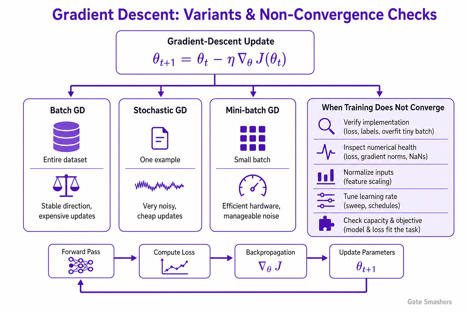
The parameter vector θ moves opposite to the gradient of objective J. The learning rate η controls the step size.
| Variant | Examples per update | Main trade-off |
|---|---|---|
| Batch | Entire training set | Stable direction but expensive updates |
| Stochastic | One example | Very noisy but cheap individual updates |
| Mini-batch | Small batch | Efficient hardware use with manageable noise |
How the update works
At the current parameter vector, the gradient indicates the local direction of greatest increase in the objective. Moving in the negative-gradient direction should reduce the loss for a sufficiently small step. Training repeats forward computation, loss calculation, backpropagation and parameter updates.
Main variants
- Batch gradient descent: Computes each update from the full training set. The direction is stable but each step can be expensive.
- Stochastic gradient descent: Updates from one example. It is noisy and inexpensive per step, but hardware utilization may be poor.
- Mini-batch gradient descent: Uses a batch of examples. It balances gradient noise, throughput and memory use and is standard for neural networks.
Learning-rate behaviour
A learning rate that is too large can cause oscillation, divergence or NaN values. A rate that is too small creates slow progress or apparent plateaus. Schedules such as warm-up, decay or cosine annealing alter the step size during training. Adaptive optimizers such as Adam maintain running estimates of gradient moments, but they do not remove the need to tune the learning rate or validate generalization.
Debugging non-convergence
- Verify the implementation: Test the loss, labels, masking and a tiny batch that the model should be able to overfit.
- Inspect numerical health: Track loss, gradient norms, parameter norms, NaNs and exploding or vanishing activations.
- Normalize inputs: Features on radically different scales can make optimization difficult.
- Tune the step: Sweep learning rates before changing many other settings.
- Check capacity and objective: Optimization cannot fix a model that cannot represent the pattern or a loss that does not match the task.
Important interview point
Gradient descent finds a useful minimum; it does not guarantee the global minimum for general non-convex objectives. In modern deep learning, optimization quality and generalization quality are related but not identical.
05What is data leakage in machine learning? Explain different types with examples and a prevention strategy.
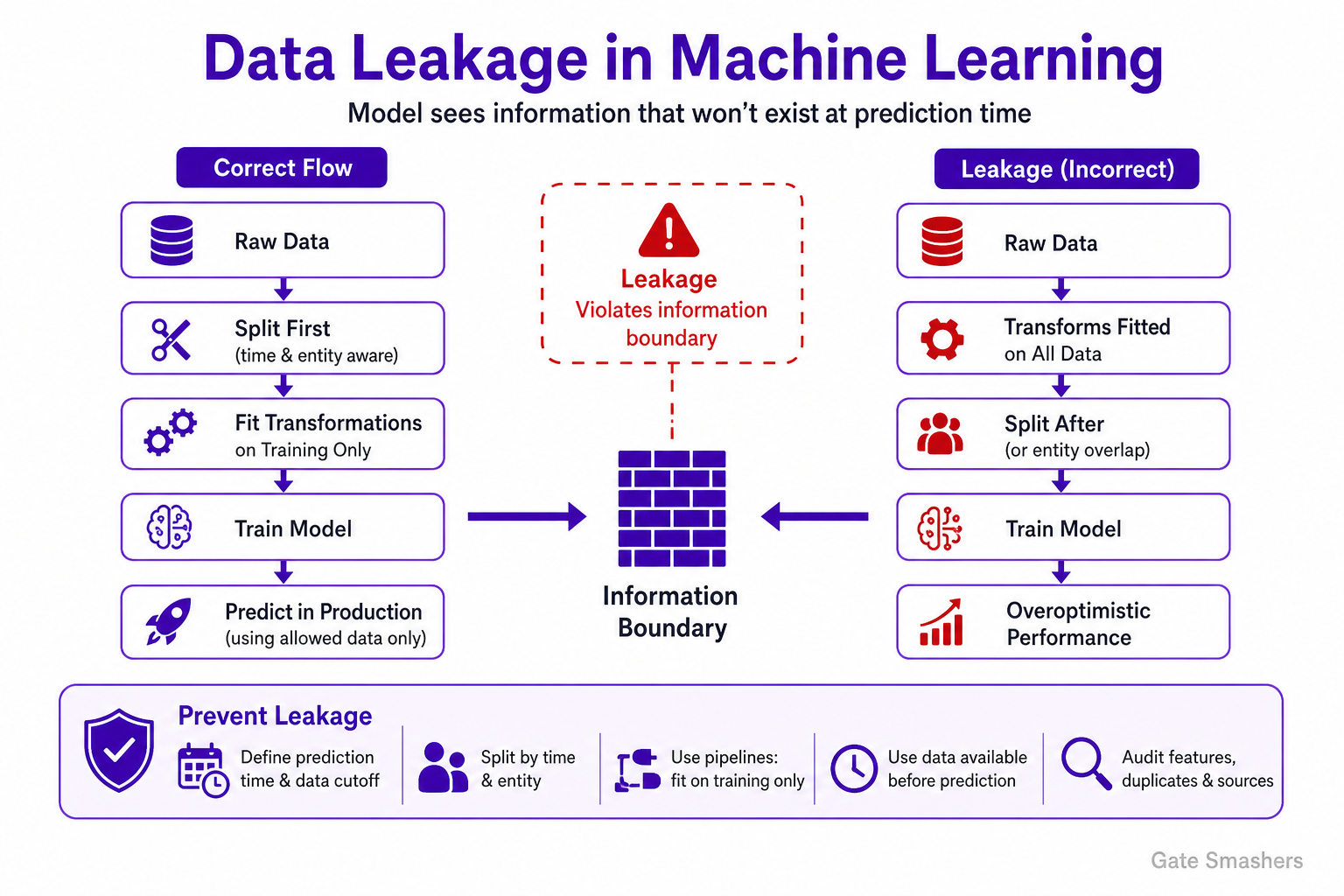
Data leakage occurs when training uses information that would not be legitimately available when the model makes a real prediction, or when held-out data influences training. Typical cases include target leakage, future leakage, preprocessing before splitting, duplicate entities across splits and test-set-driven tuning. I prevent it by defining the prediction timestamp, splitting raw data first, fitting transformations inside training-only pipelines and auditing every feature’s source and availability.
| Leakage type | Example | Prevention |
|---|---|---|
| Target / post-outcome | Using a field recorded after the outcome | Enforce a prediction-time feature cutoff |
| Future / look-ahead | Future observations enter a rolling feature | Use time-aware windows and tests |
| Preprocessing | Scaler fitted on all data | Fit transformations inside each training fold |
| Entity overlap | Same customer appears in train and test | Group-aware splitting |
| Test tuning | Threshold selected using test results | Tune on validation data only |
from sklearn.pipeline import Pipeline
from sklearn.impute import SimpleImputer
from sklearn.preprocessing import StandardScaler
from sklearn.linear_model import LogisticRegression

model = Pipeline([
    ("imputer", SimpleImputer(strategy="median")),
    ("scaler", StandardScaler()),
    ("classifier", LogisticRegression())
])

# The pipeline learns imputation and scaling only from X_train.
model.fit(X_train, y_train)
score = model.score(X_validation, y_validation)Leakage is an information-boundary failure
A feature may be strongly correlated with the target and still be invalid. The key question is whether that value exists, in the same form, at the moment the production prediction is made. Leakage can also happen without an obviously suspicious feature when preprocessing or data selection uses held-out information.
Types and examples
- Target leakage: A hospital readmission model uses a discharge field that is recorded after the prediction should occur.
- Look-ahead leakage: A demand forecast uses a rolling average that accidentally includes future days.
- Train–test contamination: The same customer or near-duplicate document appears in both sets.
- Transformation leakage: A scaler, imputer or feature selector is fitted on the complete dataset.
- Label leakage through proxies: A feature such as ‘refund processed’ nearly encodes the fraud label because it happens after investigation.
- Evaluation leakage: Test performance guides model selection or decision-threshold tuning.
Prevention checklist
- Write down the prediction event, prediction timestamp and allowed data sources.
- Split at the entity and time level before fitting any learned transformation.
- Put preprocessing, feature selection and the estimator in one reproducible pipeline.
- Compute aggregates using only data available before each prediction timestamp.
- Search for duplicates and near-duplicates across splits.
- Ask domain experts when every feature becomes available operationally.
- Keep a final untouched test set and reproduce features using production-like code.
How leakage differs from overfitting
Overfitting learns unstable patterns from legitimate training information. Leakage gives the model illegitimate information. Both may create a train–validation mismatch, but regularization cannot repair a leaked evaluation design.
Common mistake
Dropping one suspicious column is not a complete leakage audit. Leakage may be hidden in timestamps, aggregates, preprocessing state, labels, sampling rules or duplicated entities.
06In an imbalanced classification problem, how do you choose between precision and recall, and how do you select the decision threshold?
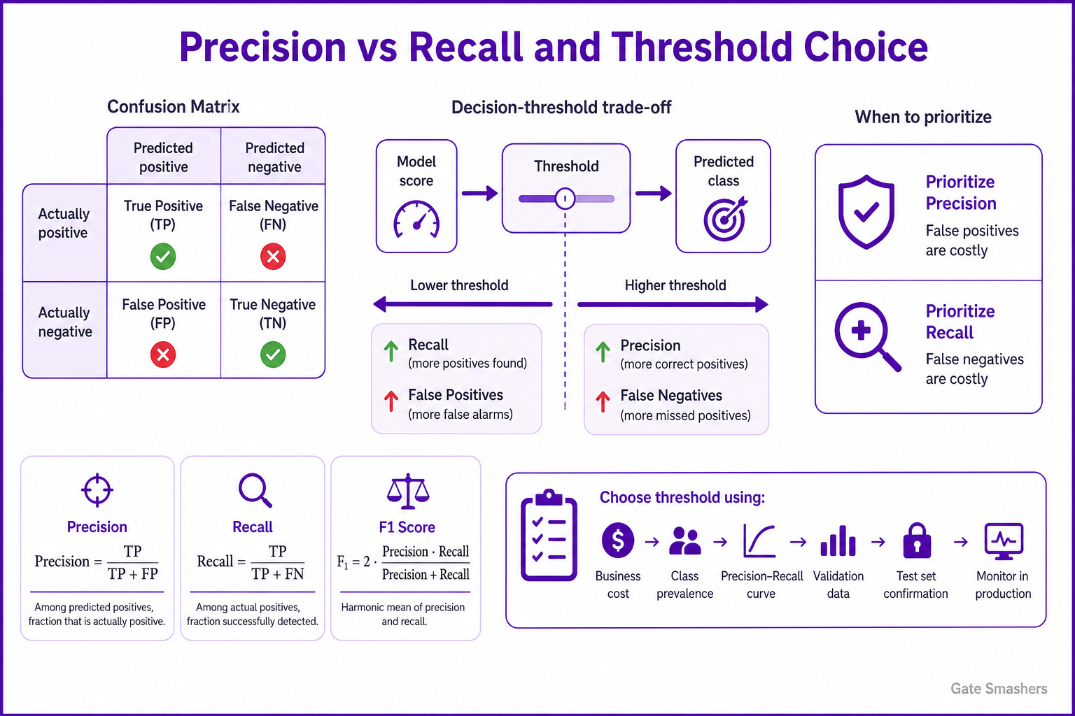
Precision measures how many predicted positives are correct, while recall measures how many actual positives are found. I prioritize precision when false positives are expensive and recall when false negatives are expensive. I do not choose the metric or threshold from accuracy alone; I use the business cost, class prevalence, a precision–recall curve and validation data, then confirm the selected threshold on an untouched test set and monitor it in production.
| Predicted positive | Predicted negative | |
|---|---|---|
| Actually positive | True Positive (TP) | False Negative (FN) |
| Actually negative | False Positive (FP) | True Negative (TN) |
Among predicted positives, precision is the fraction that is actually positive.
Among actual positives, recall is the fraction successfully detected.
F1 is the harmonic mean of precision and recall. It is useful when both matter, but it does not encode every business cost.
Start with the confusion matrix
Precision and recall describe different errors. Precision decreases when false positives increase. Recall decreases when false negatives increase. The correct priority therefore depends on the consequence of each error, not on a universal rule.
Scenario-based choice
- Spam filtering: Excessive false positives may hide legitimate mail, so precision can be especially important.
- Serious-disease screening: Missing a positive case may be costly, so high recall is often prioritized, followed by a confirmatory test.
- Fraud investigation: The operating point must balance recovered fraud against the limited capacity of investigators and customer friction.
- Search or recommendations: Precision@K and Recall@K may be more meaningful than unrestricted binary metrics because only a ranked shortlist is shown.
Threshold selection
A classifier score is converted into a class by a threshold. Lowering the threshold usually increases recall and false positives; raising it usually increases precision and false negatives. Choose the threshold on validation data by optimizing a stated constraint or utility, such as maximum recall while maintaining precision above 90%, or minimum expected business cost.
Why accuracy can mislead
If only 1% of examples are positive, predicting every example as negative produces 99% accuracy and zero recall. Always inspect prevalence, the confusion matrix and metrics that reflect the actual decision.
Production considerations
Precision changes when class prevalence changes, even if the score distributions are otherwise similar. Monitor calibration, prevalence, threshold-specific metrics and delayed labels. Revisit the threshold when costs, capacity or the data distribution changes.
07Compare a decision tree, random forest and gradient boosting. When would you choose each one?
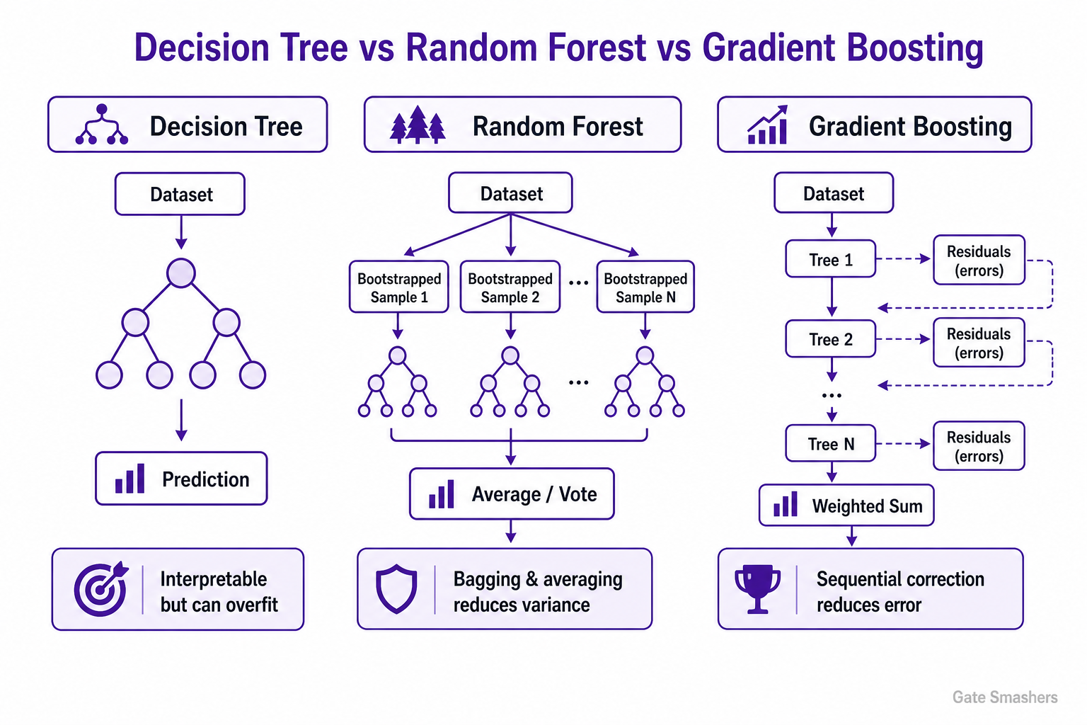
A decision tree is interpretable and fast but can overfit. A random forest trains many trees independently on bootstrapped data and random feature subsets, then averages them to reduce variance. Gradient boosting builds trees sequentially so each stage corrects the current model’s errors, often achieving stronger tabular-data accuracy but requiring careful tuning. I choose based on interpretability, accuracy, latency, data size and operational constraints, then validate rather than assuming one method always wins.
| Property | Decision Tree | Random Forest | Gradient Boosting |
|---|---|---|---|
| Interpretability | High when shallow | Lower | Lower |
| Overfitting risk | High when deep | Reduced by averaging | Controlled through shrinkage and regularization |
| Training | Single model | Independent trees | Sequential trees |
| Typical use | Explainable baseline | Robust nonlinear baseline | High-quality tabular model |
Decision tree
A decision tree recursively splits the feature space to reduce impurity or prediction error. Its rule path is easy to inspect, and it handles nonlinear interactions without feature scaling. A deep tree, however, can change substantially with small data changes and overfit the training set.
Random forest
A random forest applies bagging. Each tree is trained on a bootstrap sample and considers a random subset of features at each split. Trees are trained largely independently, and their predictions are averaged or voted. This decorrelates errors and reduces variance compared with one deep tree.
Gradient boosting
Boosting adds weak learners sequentially. Each new tree is fitted to improve the current ensemble according to the loss gradient. Libraries such as XGBoost, LightGBM and CatBoost include regularization and systems optimizations. Boosting often performs extremely well on structured data but is more sensitive to depth, learning rate, number of trees, leakage and noisy labels.
Choosing in practice
- Choose a small decision tree when a transparent rule set or very low inference complexity is more important than maximum accuracy.
- Choose a random forest for a robust nonlinear baseline with limited tuning and parallel training.
- Choose gradient boosting when tabular predictive performance is the priority and careful validation and tuning are available.
- Consider calibration, model size, feature availability, missing values, latency and explanation requirements before deployment.
Important interview point
Random forest mainly reduces variance through independent trees and averaging. Gradient boosting mainly reduces residual error through sequential correction. Neither automatically solves class imbalance, leakage or distribution shift.
08A model had strong offline performance but its production performance has dropped. How would you diagnose and recover the system?
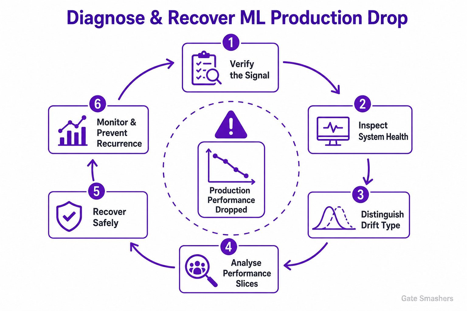
I would first confirm the drop is real by checking metric definitions, label delay, logging and pipeline health. Then I would separate data quality issues, training–serving skew, data or concept drift, threshold and calibration changes, and upstream product changes. I would compare production and training distributions by feature and segment, inspect errors with fresh labels, mitigate safely through rollback or fallback rules, and retrain only after identifying the cause and validating the replacement model.
| Failure class | Evidence to inspect | Typical response |
|---|---|---|
| Measurement issue | Metric code, labels, joins, attribution window | Repair measurement before model changes |
| Data quality | Missingness, range, freshness, schema | Fix pipeline and backfill safely |
| Training–serving skew | Offline vs online feature values | Unify feature logic and redeploy |
| Data / concept drift | Feature distributions and labelled slice metrics | Recalibrate, retrain or redesign |
| Service issue | Latency, timeouts, fallback and version mix | Rollback or restore dependency health |
PSI is one possible summary of distribution change between reference proportions pᵢ and current proportions qᵢ. Thresholds are context-dependent and PSI alone does not prove concept drift.
Step 1: verify the signal
A dashboard change is not automatically a model failure. Confirm that the same metric, population, attribution window and label definition are being compared. Check whether recent labels are incomplete and whether instrumentation or joins changed.
Step 2: inspect system health
- Feature pipeline: Missing values, stale features, schema changes, unit changes and incorrect defaults.
- Training–serving skew: Different preprocessing, encodings or feature definitions between offline and online paths.
- Service behaviour: Timeouts, fallback rates, model-version mix, latency and dependency failures.
- Product changes: A new UI, policy, campaign or traffic source can alter who receives predictions and how they respond.
Step 3: distinguish drift types
Data drift means the input distribution changes. Label shift means changes. Concept drift means the relationship changes. Feature-distribution tests can detect some input changes, but labelled outcome data is usually needed to confirm degradation in the predictive relationship.
Step 4: analyse performance slices
Compare cohorts by geography, device, acquisition channel, model score, class, time and other meaningful segments. Inspect fresh false positives and false negatives. A global average can hide a severe failure in one high-value segment.
Step 5: recover safely
Rollback a faulty release, repair the feature pipeline, apply a safe fallback or adjust traffic if users are at risk. Retrain with recent representative data only after verifying labels and leakage boundaries. Shadow-test and canary the replacement model before a full rollout.
Prevention
Monitor feature quality, prediction distributions, calibration, business outcomes, latency and model versions. Record data and model lineage, define alert thresholds and maintain rollback and retraining playbooks. Automatic retraining should still have quality gates; blindly retraining on corrupted data can make the incident worse.
09Design a recommendation system end to end. How would you generate candidates, rank them, evaluate quality and handle cold start?
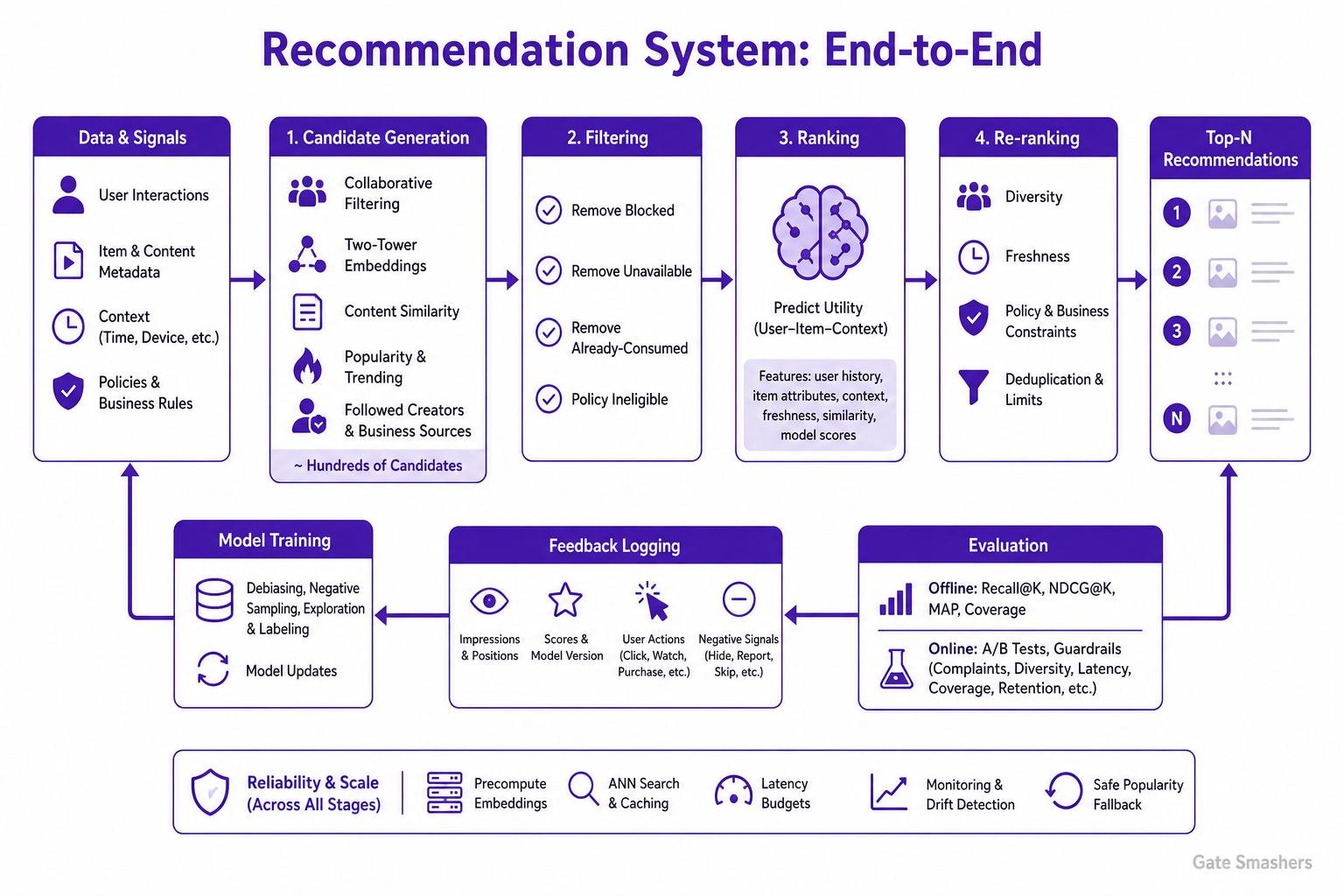
I would use a multi-stage system: collect consented interaction and item data, generate a few hundred candidates using collaborative, content-based and popularity sources, filter ineligible items, rank candidates with a model using user, item and context features, then apply diversity, freshness and policy rules. I would evaluate retrieval and ranking offline, validate impact through controlled online experiments, and monitor latency, coverage, feedback loops and segment quality. Cold-start users and items need metadata, popularity, exploration and onboarding signals.
Recall@K measures how many relevant items were retrieved in the top K candidates.
NDCG rewards relevant items near the top of a ranked list and normalizes by the ideal ordering.
| Stage | Purpose | Typical methods |
|---|---|---|
| Candidate generation | Reduce a large catalog to hundreds of items | Two-tower retrieval, collaborative filtering, similarity, popularity |
| Eligibility filtering | Remove invalid or unsafe items | Availability, policy, block and history rules |
| Ranking | Estimate utility and order candidates | Learning-to-rank, classification or regression models |
| Re-ranking | Apply list-level quality and constraints | Diversity, freshness, deduplication, quotas |
Begin with the objective
Define the recommendation surface and success event before selecting an algorithm. Watch time, click-through rate, purchase probability, retention and user satisfaction lead to different systems. Include guardrails such as complaints, hides, cancellations, diversity and latency so the model does not optimize a narrow proxy at the expense of users.
Candidate generation
Retrieving from the full catalog at request time is usually too expensive. Candidate generators produce a manageable set using methods such as item-to-item similarity, collaborative filtering, two-tower embeddings, content similarity, recent popularity, followed creators and business-specific sources. Multiple generators improve coverage.
Filtering and ranking
Remove blocked, unavailable, already-consumed or policy-ineligible items. A ranking model then predicts utility for each user–item–context tuple. Features may include user history, item attributes, freshness, similarity, context and calibrated outputs from other models. A final re-ranking stage can enforce diversity, freshness, deduplication, creator limits and business constraints.
Feedback and training data
Log impressions, positions, scores, model versions and subsequent actions. Clicks are exposure-biased: an item cannot be clicked if it was never shown, and position affects the probability of interaction. Negative sampling, debiasing, exploration and carefully defined labels are essential.
Cold start
- New user: Use onboarding interests, location or context where appropriate, popular high-quality items and controlled exploration.
- New item: Use metadata and content embeddings, creator information and a small exploration budget.
- Sparse domain: Blend collaborative signals with content and popularity rather than relying on a single method.
Evaluation
Offline retrieval metrics include Recall@K and coverage. Ranking metrics include NDCG@K, MAP and calibrated task metrics. Offline improvements are not sufficient: run A/B tests with primary and guardrail metrics, and inspect new-user and long-tail segments.
Reliability and scale
Precompute embeddings and indexes, cache stable candidates, use approximate nearest-neighbour search, set latency budgets for each stage and provide a safe popularity fallback. Monitor catalog coverage, score drift, repeated content, delayed feedback, filter rates and online outcomes.
10How would you build and operate a machine-learning system end to end, from problem definition to reliable production monitoring?
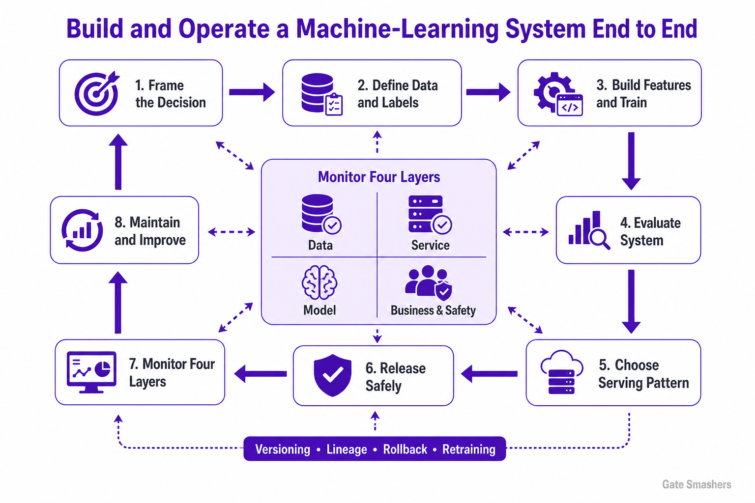
I would start with the business decision, users, constraints and measurable baseline; define labels and prediction-time features; build reproducible data and validation pipelines; train and evaluate candidate models with leakage-safe splits; package preprocessing with the model; deploy through shadow or canary stages; and monitor data quality, service health, model quality and business outcomes. I would also maintain versioning, lineage, rollback, retraining criteria and human review for high-risk decisions.
| Phase | Primary output | Critical check |
|---|---|---|
| Problem framing | Decision, objective, constraints and baseline | Metric matches real value |
| Data | Versioned dataset, labels and features | Prediction-time availability and no leakage |
| Training | Reproducible model pipeline | Tracked inputs, code and parameters |
| Evaluation | Offline and slice-level report | Untouched test and guardrails |
| Deployment | Versioned serving artefact | Shadow/canary checks and rollback |
| Monitoring | Data, service, model and business dashboards | Actionable alerts and owners |
| Maintenance | Retraining and incident process | Quality gates before replacement |
define_problem_and_metrics()
raw_data = load_versioned_data()
train, validation, test = leakage_safe_split(raw_data)
pipeline = fit_preprocessing_and_model(train)
tune_on(validation)
freeze(pipeline)
assert_quality_gates(evaluate(pipeline, test))
shadow_deploy(pipeline)
canary_release(pipeline)
monitor(data, service, model, business)
rollback_or_retrain_when_policy_triggers()1. Frame the decision
Specify who or what receives a prediction, when it is made, what action follows and what failure costs. Translate the business goal into an offline metric, online outcome and guardrail metrics. Establish a simple baseline before investing in a complex model.
2. Define labels and data boundaries
Document the prediction timestamp, label window, feature availability and entity keys. Build data-quality checks for schema, missingness, ranges, duplicates and freshness. Use time-aware or group-aware splits when the deployment setting requires them.
3. Build reproducible features and training
Keep transformation logic versioned and, where possible, shared between training and serving. Track dataset snapshots, code, features, hyperparameters, random seeds, metrics and model artefacts. Automate training through repeatable pipelines rather than notebook-only steps.
4. Evaluate the complete system
Compare with baselines and evaluate the metric that matches the decision. Inspect calibration, latency, fairness or safety constraints, robustness and performance slices. Tune on validation data and use an untouched test set for the frozen pipeline.
5. Choose a serving pattern
Design for feature freshness, throughput, latency, fallback behaviour and model-version compatibility.
- Batch inference: Appropriate when predictions can be computed periodically and latency is not immediate.
- Online inference: Appropriate when current context is required and request latency matters.
- Streaming inference: Appropriate when event-driven updates or near-real-time state are required.
6. Release safely
Validate the artefact, run integration tests and compare online features with offline expectations. Use shadow deployment to observe behaviour without affecting users, then canary or A/B rollout with automated and human-monitored guardrails. Maintain a rollback path.
7. Monitor four layers
- Data: Schema, freshness, missingness, ranges and distribution shift.
- Service: Availability, throughput, latency, errors and fallback rate.
- Model: Prediction distribution, calibration, segment metrics and performance when labels arrive.
- Business and safety: The actual outcome, guardrails, complaints and harmful failure modes.
8. Maintain and improve
Define who owns incidents, what triggers investigation or retraining and which approval gates a replacement must pass. Retraining may be scheduled, drift-triggered or performance-triggered, but every new model should be evaluated as a new release. Preserve lineage so a prediction can be traced to the data, features, code and model version that produced it.
Important interview point
A production ML system is more than a model endpoint. Data contracts, feature correctness, experimentation, deployment safety, monitoring and operational ownership usually determine whether the system creates lasting value.